Getting started tutorial
[ ]:
%pip install --upgrade --quiet pip
%pip install --upgrade --quiet circuitree==0.11.1 numpy matplotlib tqdm ipympl ffmpeg moviepy watermark
Problem statement
CircuiTree solves the following problem:
Given a phenotype that can be simulated, a reward function that measures the phenotype, and a space of possible circuit architectures, find the optimal architecture(s) to achieve that target phenotype by running a reasonable number of simulations.
In order to solve this problem, CircuiTree uses a search algorithm called Monte Carlo tree search (MCTS), borrowed from artificial intelligence and reinforcement learning, to search over the space of possible architectures, or topologies. MCTS is an algorithm for planning and game-playing, so we approach circuit design as a game of stepwise assembly, where each step adds an interaction to the circuit diagram.
The main class provided by this package is CircuiTree, and to run a tree search, the user should make their own subclass of CircuiTree that defines (1) a space of possible topologies to search and (2) a reward function that returns a (possibly stochastic) estimate of phenotypic quality.
Creating a CircuiTree class
[2]:
from circuitree import CircuiTree
Let’s consider a simple example. Say we are interested in constructing a circuit of three transcription factors (TFs) A, B, and C that exhibits bistability, where the system can be “switched” from one state (e.g. high A, low B) to another (high B, low A). We will allow each TF to activate or inhibit any of the TFs (including itself). Multiple regulation (A both activates and inhibits B) is not allowed. With these rules, we have defined a set of topologies (a design space) that we are sampling from.
[3]:
components = ["A", "B", "C"] # Three transcription factors (TFs)
interactions = [
    "activates", # Each pairwise interaction has two options
    "inhibits",
]
CircuiTree explores the design space by treating circuit design as a game where the topology is built step-by-step, and the objective is to assemble the best circuit. Specifically, CircuiTree represents each circuit topology as a string called a state, and it can choose from a list of actions that either change the state or terminate the assembly process (i.e. “click submit” on the game). The algorithm searches starting from a “root” state, and over many iterations it builds a
decision tree of candidate topologies and preferentially explores regions of that tree with higher mean reward.
1. Choose a Grammar
The rules for how states are defined and how they are affected by taking actions (i.e. the rules of the game) are called a “grammar.” We will be using the built-in SimpleNetworkGrammar class to explore the design space we defined above. (See the grammar tutorial for more details on grammars and how to define custom design spaces from the base CircuitGrammar class.)
[4]:
# Built-in grammars can be found in the `models` module
from circuitree.models import SimpleNetworkGrammar

grammar = SimpleNetworkGrammar(
    components=components,
    interactions=interactions,
)
2. Define a reward function
The only strict requirement for the reward function is that it should return bounded values, ideally between 0 and 1. NOTE: If reward values have a larger range, you may need to increase the exploration_constant argument proportionally.
For our test case, bistability is known to require positive feedback. For example, positive autoregulation (A activates itself) or mutual inhibition (A inhibits B and B inhibits A). Here we will use a dummy reward function that doesn’t actually compute bistability but instead just looks for the presence of positive feedback loops. The reward value will be a random number drawn from a Gaussian distribution, and we will increase the mean of that distribution for every type of positive feedback
loop the topology contains. In a real scenario, the reward function might be more complex, possibly requiring multiple simulations. To mimic the computational cost of a costly evaluation, we’ll introduce an optional argument expensive that pauses for 0.1 seconds before returning the result.
[5]:
from time import sleep
import numpy as np

def get_bistability_reward(state, grammar, rg=None, expensive=False):
    """Returns a reward value for the given state (topology) based on
    whether it contains positive-feedback loops (PFLs). Assumes the
    state is a string in the format of SimpleNetworkGrammar."""

    # We list all types of PFLs with up to 3 components. Each three-letter
    # substring is an interaction in the circuit, and interactions are
    # separated by underscores.
    patterns = [
        "AAa",  # PAR - "AAa" means "A activates A"
        "ABi_BAi",  # Mutual inhibition - "A inhibits B, B inhibits A"
        "ABa_BAa",  # Mutual activation
        "ABa_BCa_CAa",  # Cycle of all activation
        "ABa_BCi_CAi",  # Cycle with two inhibitions
    ]

    # Mean reward increases with each PFL found (from 0.25 to 0.75)
    mean = 0.25
    for pattern in patterns:

        # The "has_pattern" method returns whether state contains the pattern.
        # It checks all possible renamings. For example, `has_pattern(s, 'AAa')`
        # checks whether the state `s` contains 'AAa', 'BBa', or 'CCa'.
        if grammar.has_pattern(state, pattern):
            mean += 0.1

    if expensive: # Simulate a more expensive reward calculation
        sleep(0.1)

    # Use the default random number generator if none is provided
    rg = np.random.default_rng() if rg is None else rg

    return rg.normal(loc=mean, scale=0.1)
3. Create a subclass
Our subclass of CircuiTree must define the get_reward method. The first argument of the method should be a state, or unique identifier corresponding to a topology. For many features, the method is_success should also be defined. It should take the name of a terminal topology and return True if it is considered “successful” overall at generating the phenotype.
We will say that a successfully bistable circuit should have a mean reward of >0.5, which we will calculate empirically as the cumulative reward divided by the number of samples, or “visits” to that state.
[6]:
class BistabilityTree(CircuiTree):
    """A subclass of CircuiTree that searches for positive feedback networks.
    Uses the SimpleNetworkGrammar to encode network topologies. The grammar can
    be accessed with the `self.grammar` attribute."""

    def __init__(self, *args, **kwargs):
        kwargs = kwargs | {"grammar": grammar}
        super().__init__(*args, **kwargs)

    def get_reward(self, state: str, expensive: bool = False) -> float:
        """Returns a reward value for the given state (topology) based on
        whether it contains positive-feedback loops (PFLs)."""

        # `self.rg` is a Numpy random generator that can be seeded on initialization
        reward = get_bistability_reward(
            state, self.grammar, self.rg, expensive=expensive
        )
        return reward

    def get_mean_reward(self, state: str) -> float:
        """Returns the mean empirical reward value for the given state."""
        # The search graph is stored as a `networkx.DiGraph` in the `graph`
        # attribute. We can access the cumulative reward and # of visits for
        # each node (state) using the `reward` and `visits` attributes.
        return (
          self.graph.nodes[state].get("reward", 0)
          / self.graph.nodes[state].get("visits", 1)
        )

    def is_success(self, state: str) -> bool:
        """Returns whether a topology is a successful bistable circuit design."""
        if self.grammar.is_terminal(state):
            return self.get_mean_reward(state) > 0.5
        else:
            return False # Ignore incomplete topologies
Running a tree search
We can run a search using the CircuiTree.search_mcts() method (or CircuiTree.search_mcts_parallel() for a parallel search). We need to supply a “root” state string that is the initial state of the assembly game, in this case a circuit with three TFs (A, B, and C) and no interactions. Using the SimpleNetwork format, this is represented by the string ABC::. We can specify any additional keyword arguments for the reward functions using the run_kwargs argument.
[7]:
# Make an instance of the search tree
tree = BistabilityTree(
    grammar=grammar,
    root="ABC::", # The root state - 3 TFs, no interactions
    seed=0, # Seed for the random number generator
)

# Run the search
tree.search_mcts(
    n_steps=50_000,
    progress_bar=True,
    run_kwargs={"expensive": False}
)
MCTS search: 1%| | 422/50000 [00:00<00:29, 1688.86it/s]
Starting MCTS search with 50000 iterations.
MCTS search: 100%|██████████| 50000/50000 [01:07<00:00, 745.51it/s]
Visualizing results
The best individual topologies
To get an initial feel for the results, let’s plot the 10 designs with the highest average reward after filtering out the states with 10 or fewer samples.
[8]:
import matplotlib.pyplot as plt
from circuitree.viz import plot_network

%matplotlib inline

# Top 10 designs with at least 10 visits
def robustness(state):
    r = tree.graph.nodes[state].get("reward", 0)
    v = tree.graph.nodes[state].get("visits", 1)
    return r / v

# Recall that only the "terminal" states are fully assembled circuits
states = [s for s in tree.terminal_states if tree.graph.nodes[s]["visits"] > 10]
top_10_states = sorted(states, key=robustness, reverse=True)[:10]

# Plot the top 10
fig = plt.figure(figsize=(12, 5))
plt.suptitle("Top 10 bistable circuits and their robustness")
for i, state in enumerate(top_10_states):
    ax = fig.add_subplot(2, 5, i + 1)

    # The `viz.plot_network()` function plots SimpleNetwork-formatted strings
    plot_network(
        *grammar.parse_genotype(state),
        ax=ax,
        plot_labels=False,
        node_shrink=0.6,
        auto_shrink=0.8,
        offset=0.75,
        padding=0.4
    )
    r = tree.graph.nodes[state]["reward"]
    v = tree.graph.nodes[state]["visits"]
    ax.set_title(f"{r / v:.2f} (n={v})")
    ax.set_xlim(-1.5, 1.5)
    ax.set_ylim(-1.0, 1.8)
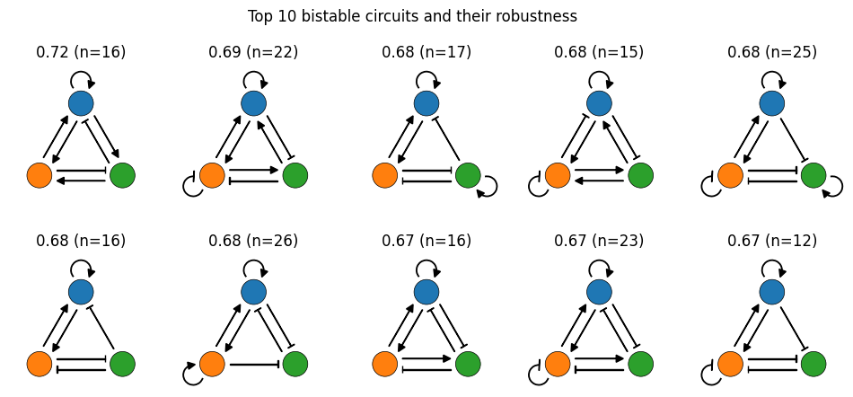
Recall that our reward function is counting the number of different positive feedback loops. By that standard, our best solutions are great! Most contain 3 or 4 different PFLs.
Overall sampling of the search graph
To visualize where the search allocated its samples over the whole search space, we can view the whole search graph at once using a complexity layout.
[9]:
from circuitree.viz import plot_complexity

# Plotting options
plot_kwargs = dict(
    tree=tree,
    aspect=1.5,
    alpha=0.25,
    n_to_highlight=10,  # number of top states to highlight
    highlight_min_visits=10,  # only highlight states with 10+ visits
)
min_visits_per_move = 10

## Plot
fig = plt.figure(figsize=(13, 5))
plt.suptitle("Search space for the Bistability game")

ax1 = fig.add_subplot(1, 2, 1)
plt.title("All moves")
plot_complexity(fig=fig, ax=ax1, **plot_kwargs)

ax2 = fig.add_subplot(1, 2, 2)
plt.title(f"Moves with {min_visits_per_move}+ visits")
plot_complexity(vlim=(min_visits_per_move, None), fig=fig, ax=ax2, **plot_kwargs)
[9]:
(<Figure size 1300x500 with 2 Axes>,
 <Axes: title={'center': 'Moves with 10+ visits'}, ylabel='Complexity'>)
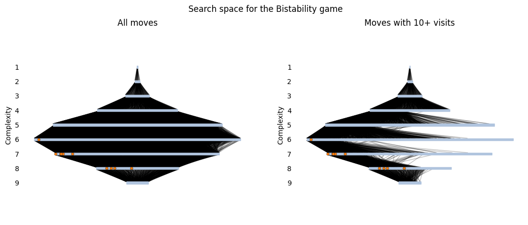
In a complexity layout, terminal topologies are arranged into layers based on their complexity, or the number of interactions in the circuit diagram. The width of the layer represents the number of topologies with that complexity, and topologies within a layer are sorted from most visited to least visited during the search. A line from a less complex topology \(s_i\) to a more complex one \(s_j\) indicates that the assembly move \(s_i \rightarrow s_j\) was visited at least once (left) or at least ten times (right). Finally, we use orange circles to highlight the top 10 topologies shown above.
The graph on the left shows that the overall space is quite well sampled. In all the layers, even the least-visited states (on the right of each layer) have many incoming and outgoing edges, showing that many options were explored. If we only look at the moves with 10+ visits, the graph on the right shows that the search favored a subset of the overall graph that has a higher concentration of top solutions. This is great! It means that our search struck a good balance between exploring the overall space and focusing samples on high-reward areas.
Animating the search
To make a video of the search process, we will re-run the search, this time saving the tree object every 1,000 steps. To do that, we’ll create a callback function that saves the tree to file. A callback is a function that is passed as an input to another function. If you supply the callback and callback_every arguments, search_mcts() will call your callback periodically during search. We can use callbacks to perform periodic backups, save progress metrics, or end the search early
if a stopping condition is reached.
[10]:
# # Remember to delete the backup folder before re-running this cell!
# # Otherwise, the video may contain multiple runs
# !rm -r ./tree-backups

from pathlib import Path
from datetime import datetime

today = datetime.now().strftime("%y%m%d")

# Make a folder for backups
save_dir = Path("./tree-backups")
save_dir.mkdir(exist_ok=True)

## Callbacks should have the following call signature:
##       callback(tree, iteration, selection_path, simulated_node, reward)
## We only need the first two arguments to do a backup.
def save_tree_callback(tree: BistabilityTree, iteration: int, *args, **kwargs):
    """Saves the BistabilityTree to two files, a `.gml` file containing the
    graph and a `.json` file with the other object attributes."""
    gml_file = save_dir.joinpath(f"{today}_bistability_search_{iteration}.gml")
    json_file = save_dir.joinpath(f"{today}_bistability_search_{iteration}.json")
    tree.to_file(gml_file, json_file)

# Redo the search with periodic backup
n_steps = 50_001
tree = BistabilityTree(grammar=grammar, root="ABC::")
tree.search_mcts(
    n_steps=n_steps,
    progress_bar=True,
    run_kwargs={"expensive": False},
    callback=save_tree_callback,
    callback_every=500,
    callback_before_start=False,
)
print("Search complete!")
MCTS search: 0%| | 206/50001 [00:00<00:24, 2055.06it/s]
Starting MCTS search with 50001 iterations.
MCTS search: 100%|██████████| 50001/50001 [01:21<00:00, 614.11it/s]
Search complete!
Then, we can make the video using matplotlib’s animation interface. This might take a few minutes to run.
[11]:
from matplotlib.animation import FuncAnimation

# Load the saved data in order of iteration
gml_files = sorted(save_dir.glob("*.gml"), key=lambda f: int(f.stem.split("_")[-1]))
json_files = sorted(save_dir.glob("*.json"), key=lambda f: int(f.stem.split("_")[-1]))
iterations = [int(f.stem.split("_")[-1]) for f in gml_files]

# Make an animation from each saved time-point
anim_dir = Path("./animations")
anim_dir.mkdir(exist_ok=True)

fig = plt.figure(figsize=(13, 5))
ax1 = fig.add_subplot(1, 2, 1)
ax1.set_title("All moves")
ax2 = fig.add_subplot(1, 2, 2)
ax2.set_title("Moves with 10+ visits")

def render_frame(f: int):
    """Render frame `f` of the animation."""
    ax1.clear()
    ax2.clear()

    tree = BistabilityTree.from_file(
        gml_files[f], json_files[f], grammar_cls=SimpleNetworkGrammar
    )

    plt.suptitle(f"Iteration {iterations[f]}")
    ax1.set_title("All moves")
    ax2.set_title("Moves with 10+ visits")
    plot_complexity(fig=fig, ax=ax1, tree=tree, aspect=1.5, alpha=0.25)
    plot_complexity(
        fig=fig,
        ax=ax2,
        tree=tree,
        aspect=1.5,
        alpha=0.25,
        vlim=(10, None),
    )

# Make the animation
anim = FuncAnimation(fig, render_frame, frames=len(gml_files))
anim_file = anim_dir.joinpath(f"{today}_bistability.mp4")

# Save the animation
anim.save(
    anim_file,
    writer="ffmpeg",
    fps=10,
    progress_callback=lambda i, n: print(f"{i + 1} / {n}")
)
print(f"Saved to: {anim_file}")

plt.close(fig)
1 / 101
2 / 101
3 / 101
4 / 101
5 / 101
6 / 101
7 / 101
8 / 101
9 / 101
10 / 101
11 / 101
12 / 101
13 / 101
14 / 101
15 / 101
16 / 101
17 / 101
18 / 101
19 / 101
20 / 101
21 / 101
22 / 101
23 / 101
24 / 101
25 / 101
26 / 101
27 / 101
28 / 101
29 / 101
30 / 101
31 / 101
32 / 101
33 / 101
34 / 101
35 / 101
36 / 101
37 / 101
38 / 101
39 / 101
40 / 101
41 / 101
42 / 101
43 / 101
44 / 101
45 / 101
46 / 101
47 / 101
48 / 101
49 / 101
50 / 101
51 / 101
52 / 101
53 / 101
54 / 101
55 / 101
56 / 101
57 / 101
58 / 101
59 / 101
60 / 101
61 / 101
62 / 101
63 / 101
64 / 101
65 / 101
66 / 101
67 / 101
68 / 101
69 / 101
70 / 101
71 / 101
72 / 101
73 / 101
74 / 101
75 / 101
76 / 101
77 / 101
78 / 101
79 / 101
80 / 101
81 / 101
82 / 101
83 / 101
84 / 101
85 / 101
86 / 101
87 / 101
88 / 101
89 / 101
90 / 101
91 / 101
92 / 101
93 / 101
94 / 101
95 / 101
96 / 101
97 / 101
98 / 101
99 / 101
100 / 101
101 / 101
Saved to: animations/240513_bistability.mp4
Now let’s watch the video!
[12]:
import moviepy.editor

moviepy.editor.ipython_display(str(anim_file))
[12]:
[16]:
%load_ext watermark
%watermark -v -p circuitree,numpy,matplotlib,tqdm,jupyterlab,ipympl,ffmpeg,moviepy,watermark
Python implementation: CPython
Python version       : 3.10.8
IPython version      : 8.24.0

circuitree: 0.11.1
numpy     : 1.26.4
matplotlib: 3.8.4
tqdm      : 4.66.4
jupyterlab: 4.1.8
ipympl    : 0.9.4
ffmpeg    : 1.4
moviepy   : 1.0.3
watermark : 2.4.3